
Sample Analysis of NBA Play-by-Play Data
Overview
This is a sample analysis to test the viability of using play-by-play NBA data from BigDataBall.com for analysis. I’ve been looking for a source of play-by-play data that would allow me to calculate things like effective field goal percentage (eFG%) of teammates while a player is on vs. off the court. The play-by-play data that’s available at places like Basketball-Reference.com and NBA.com don’t have the necessary detail (e.g., they don’t describe who is on the court for a given play), but BigDataBall appears to. The data comes with a cost, though, so I wanted to run a sample analysis with their sample file to see if I liked the format and was willing to purchase full seasons of the data.
Given that broader objective, this analysis calculates the relative eFG% of teammates while each player is on vs. off the court for both teams in Game 4 of the 2016 NBA finals.
Note: Code can be forked from my Github repository here. Also, sorry for the poor code formatting. WordPress likes to massacre Magrittr pipe operators.
Setup
Load Packages
require(tidyverse)
require(magrittr)
require(rvest)
require(ggthemes)
require(pander)
Custom Functions
To help with the analysis, I’ll create a few functions.
The first function will filter the game’s data frame down to just the records for which a given player is on the court.
filter_on = function(df, nm = "name", h_o_a = "home") {
  if (h_o_a == "home") {
    df %>%
      filter(
        h1 == nm | h2 == nm | h3 == nm | h4 == nm | h5 == nm
      )
  } else if (h_o_a == "away") {
    df %>%
      filter(
        a1 == nm | a2 == nm | a3 == nm | a4 == nm | a5 == nm
      )
  } else {
    "Error! Select 'home' or 'away' for h_o_a."
  }
}
The next function will do the same for when a given player is off the court.
filter_off = function(df, nm = "name", h_o_a = "home") {
  if (h_o_a == "home") {
    df %>%
      filter(
        h1 != nm, h2 != nm, h3 != nm, h4 != nm, h5 != nm
      )
  } else if (h_o_a == "away") {
    df %>%
      filter(
        a1 != nm, a2 != nm, a3 != nm, a4 != nm, a5 != nm
      )
  } else {
    "Error! Select 'home' or 'away' for h_o_a."
  }
}
Since I’m interested in the shooting percentage of just the teammates while a player is on vs. off the court (in other words, I’m not interested in the player’s shooting percentage but rather just the rest of his teammates’ shooting percentages), I’ll need to filter out some records. This function will filter to just the shots attempted or made by the player’s team that were not attempted/made by the player himself.
# filters to just shots by the same team as the player by someone other than the player
filter_eFG = function(df, nm = "name", tm = "teamAbbrev")  {
  df %>%
    filter(
      team == tm,
      event_type %in% c("shot", "miss"), # want shots w/o free throws
      player != nm # want shots from teammates
    )
}
I’ll also create a function to calculate the eFG%: eFG% = (FGM + 0.5 * 3PM) / FGA.
eFG = function(df, made_col = "event_type", made_text = "shot", points_col = "points") {
  (sum(df[made_col] == made_text) + 0.5 * sum(df[points_col] == 3)) / nrow(df)
}
Finally, I’ll write a function to return the relative eFG% and a few more relevant pieces of information. I’m particularly interested in returning the number of shots attempted by teammates while a player is on/off the court. If there’s a large discrepancy, which indicates that a player is either on the court or off the court for the vast majority of the game, the relative eFG% may be unreliable due to random fluctuations. I’ll want to account for that in my analysis below.
eFGRatio = function(df, nm = "name", tm = "teamAbbrev", h_o_a = "home") {
  df_on = try(df %>% filter_on(nm, h_o_a) %>% filter_eFG(nm, tm))
  df_off = try(df %>% filter_off(nm, h_o_a) %>% filter_eFG(nm, tm))

  if (nrow(df_on) == 0) {
    # no plays that meet criteria -> return NA
    eFG_on = NA
    shots_on = NA
  } else {
    eFG_on = eFG(df_on)
    shots_on = nrow(df_on)
  }

  if(nrow(df_off) == 0) {
    # no plays that meet criteria -> return NA
    eFG_off = NA
    shots_off = NA
  } else {
    eFG_off = eFG(df_off)
    shots_off = nrow(df_off)
  }

  eFG_Ratio = eFG_on / eFG_off

  output = list(
    eFG_Ratio = eFG_Ratio, # ratio of eFG of teammates while on vs. while off court
    eFG_on = eFG_on, # eFG of teammates while player is on court
    eFG_off = eFG_off, # eFG of teammates while player is off court
    shots_on = shots_on, # number of shots by teammates while player is on court
    shots_off = shots_off # number of shots by teammates while player is off court
  )

  return(output)
}
Inputs
location_of_data = "/Users/kylewurtz/Dropbox/R/NBA Play-By-Play/Sample Analysis/Data/Sample BigDataBall" # Update!
data_file_name = "Sample_BigDataBall.csv"
Read in Sample Data Set
BigDataBall offers a free sample data set of its play-by-play data, and that’s what I’ll be working with in this file. For convenience, I’ve downloaded a copy of the data set and stored it in the repository.
df = read_csv(file.path(location_of_data, data_file_name))
## Parsed with column specification:
## cols(
##   .default = col_character(),
##   period = col_integer(),
##   away_score = col_integer(),
##   home_score = col_integer(),
##   remaining_time = col_time(format = ""),
##   elapsed = col_time(format = ""),
##   play_id = col_integer(),
##   num = col_integer(),
##   outof = col_integer(),
##   points = col_integer(),
##   shot_distance = col_integer(),
##   original_x = col_integer(),
##   original_y = col_integer(),
##   converted_x = col_double(),
##   converted_y = col_double()
## )
## See spec(...) for full column specifications.
Work
Initial Investigation
Now that I have the data read in, I’ll take a quick look at the structure of the data set before moving on with the analysis.
glimpse(df)
## Observations: 467
## Variables: 44
## $ game_id        <chr> "0041500404", "0041500404", "0041500404", "0041...
## $ data_set       <chr> "2016 Playoff", "2016 Playoff", "2016 Playoff",...
## $ date           <chr> "6/10/16", "6/10/16", "6/10/16", "6/10/16", "6/...
## $ a1             <chr> "Harrison Barnes", "Harrison Barnes", "Harrison...
## $ a2             <chr> "Draymond Green", "Draymond Green", "Draymond G...
## $ a3             <chr> "Andrew Bogut", "Andrew Bogut", "Andrew Bogut",...
## $ a4             <chr> "Klay Thompson", "Klay Thompson", "Klay Thompso...
## $ a5             <chr> "Stephen Curry", "Stephen Curry", "Stephen Curr...
## $ h1             <chr> "Richard Jefferson", "Richard Jefferson", "Rich...
## $ h2             <chr> "LeBron James", "LeBron James", "LeBron James",...
## $ h3             <chr> "Tristan Thompson", "Tristan Thompson", "Trista...
## $ h4             <chr> "J.R. Smith", "J.R. Smith", "J.R. Smith", "J.R....
## $ h5             <chr> "Kyrie Irving", "Kyrie Irving", "Kyrie Irving",...
## $ period         <int> 1, 1, 1, 1, 1, 1, 1, 1, 1, 1, 1, 1, 1, 1, 1, 1,...
## $ away_score     <int> 0, 0, 0, 0, 3, 3, 3, 4, 5, 5, 7, 7, 7, 7, 10, 1...
## $ home_score     <int> 0, 0, 0, 0, 0, 3, 3, 3, 3, 6, 6, 6, 6, 8, 8, 10...
## $ remaining_time <time> 720 secs, 720 secs, 701 secs, 700 secs, 689 se...
## $ elapsed        <time> 0 secs, 0 secs, 19 secs, 20 secs, 31 secs, 46 ...
## $ play_length    <chr> "0:00:00", "0:00:00", "0:00:19", "0:00:01", "0:...
## $ play_id        <int> 0, 1, 2, 3, 4, 5, 6, 7, 9, 11, 12, 13, 14, 15, ...
## $ team           <chr> NA, "GSW", "GSW", "GSW", "GSW", "CLE", "CLE", "...
## $ event_type     <chr> "start of period", "jump ball", "miss", "reboun...
## $ assist         <chr> NA, NA, NA, NA, "Stephen Curry", "LeBron James"...
## $ away           <chr> NA, "Andrew Bogut", NA, NA, NA, NA, NA, NA, NA,...
## $ home           <chr> NA, "Tristan Thompson", NA, NA, NA, NA, NA, NA,...
## $ block          <chr> NA, NA, NA, NA, NA, NA, NA, NA, NA, NA, NA, "Dr...
## $ entered        <chr> NA, NA, NA, NA, NA, NA, NA, NA, NA, NA, NA, NA,...
## $ left           <chr> NA, NA, NA, NA, NA, NA, NA, NA, NA, NA, NA, NA,...
## $ num            <int> NA, NA, NA, NA, NA, NA, NA, 1, 2, NA, NA, NA, N...
## $ opponent       <chr> NA, NA, NA, NA, NA, NA, "Draymond Green", NA, N...
## $ outof          <int> NA, NA, NA, NA, NA, NA, NA, 2, 2, NA, NA, NA, N...
## $ player         <chr> NA, "Tristan Thompson", "Draymond Green", "Harr...
## $ points         <int> NA, NA, 0, NA, 3, 3, NA, 1, 1, 3, 2, 0, NA, 2, ...
## $ possession     <chr> NA, "Stephen Curry", NA, NA, NA, NA, NA, NA, NA...
## $ reason         <chr> NA, NA, NA, NA, NA, NA, "s.foul", NA, NA, NA, N...
## $ result         <chr> NA, NA, "missed", NA, "made", "made", NA, "made...
## $ steal          <chr> NA, NA, NA, NA, NA, NA, NA, NA, NA, NA, NA, NA,...
## $ type           <chr> "start of period", "jump ball", "Jump Shot", "r...
## $ shot_distance  <int> NA, NA, 25, NA, 23, 24, NA, NA, NA, 23, 14, 14,...
## $ original_x     <int> NA, NA, -4, NA, 225, -240, NA, NA, NA, 232, -66...
## $ original_y     <int> NA, NA, 247, NA, -6, -19, NA, NA, NA, -11, 129,...
## $ converted_x    <dbl> NA, NA, 25.4, NA, 2.5, 1.0, NA, NA, NA, 48.2, 3...
## $ converted_y    <dbl> NA, NA, 29.7, NA, 4.4, 90.9, NA, NA, NA, 90.1, ...
## $ description    <chr> NA, "Jump Ball Thompson vs. Bogut: Tip to Curry...
summary(df)
##    game_id            data_set             date
##  Length:467         Length:467         Length:467
##  Class :character   Class :character   Class :character
##  Mode  :character   Mode  :character   Mode  :character
##
##
##
##
##       a1                 a2                 a3
##  Length:467         Length:467         Length:467
##  Class :character   Class :character   Class :character
##  Mode  :character   Mode  :character   Mode  :character
##
##
##
##
##       a4                 a5                 h1
##  Length:467         Length:467         Length:467
##  Class :character   Class :character   Class :character
##  Mode  :character   Mode  :character   Mode  :character
##
##
##
##
##       h2                 h3                 h4
##  Length:467         Length:467         Length:467
##  Class :character   Class :character   Class :character
##  Mode  :character   Mode  :character   Mode  :character
##
##
##
##
##       h5                period        away_score      home_score
##  Length:467         Min.   :1.000   Min.   :  0.0   Min.   : 0.00
##  Class :character   1st Qu.:2.000   1st Qu.: 32.0   1st Qu.:30.00
##  Mode  :character   Median :3.000   Median : 50.0   Median :55.00
##                     Mean   :2.548   Mean   : 54.7   Mean   :53.05
##                     3rd Qu.:4.000   3rd Qu.: 81.0   3rd Qu.:81.00
##                     Max.   :4.000   Max.   :108.0   Max.   :97.00
##
##  remaining_time      elapsed         play_length           play_id
##  Length:467        Length:467        Length:467         Min.   :  0.0
##  Class1:hms        Class1:hms        Class :character   1st Qu.:140.5
##  Class2:difftime   Class2:difftime   Mode  :character   Median :280.0
##  Mode  :numeric    Mode  :numeric                       Mean   :282.0
##                                                         3rd Qu.:426.5
##                                                         Max.   :583.0
##
##      team            event_type           assist
##  Length:467         Length:467         Length:467
##  Class :character   Class :character   Class :character
##  Mode  :character   Mode  :character   Mode  :character
##
##
##
##
##      away               home              block
##  Length:467         Length:467         Length:467
##  Class :character   Class :character   Class :character
##  Mode  :character   Mode  :character   Mode  :character
##
##
##
##
##    entered              left                num          opponent
##  Length:467         Length:467         Min.   :1.000   Length:467
##  Class :character   Class :character   1st Qu.:1.000   Class :character
##  Mode  :character   Mode  :character   Median :1.000   Mode  :character
##                                        Mean   :1.456
##                                        3rd Qu.:2.000
##                                        Max.   :2.000
##                                        NA's   :410
##      outof          player              points        possession
##  Min.   :1.000   Length:467         Min.   :0.0000   Length:467
##  1st Qu.:2.000   Class :character   1st Qu.:0.0000   Class :character
##  Median :2.000   Mode  :character   Median :1.0000   Mode  :character
##  Mean   :1.912                      Mean   :0.9361
##  3rd Qu.:2.000                      3rd Qu.:2.0000
##  Max.   :2.000                      Max.   :3.0000
##  NA's   :410                        NA's   :248
##     reason             result             steal
##  Length:467         Length:467         Length:467
##  Class :character   Class :character   Class :character
##  Mode  :character   Mode  :character   Mode  :character
##
##
##
##
##      type           shot_distance     original_x        original_y
##  Length:467         Min.   : 0.00   Min.   :-243.00   Min.   :-19.00
##  Class :character   1st Qu.: 2.00   1st Qu.: -84.00   1st Qu.:  1.25
##  Mode  :character   Median :14.00   Median :  -5.00   Median : 32.00
##                     Mean   :13.44   Mean   : -16.80   Mean   : 81.24
##                     3rd Qu.:24.00   3rd Qu.:  26.25   3rd Qu.:154.25
##                     Max.   :31.00   Max.   : 238.00   Max.   :257.00
##                     NA's   :305     NA's   :305       NA's   :305
##   converted_x     converted_y    description
##  Min.   : 0.70   Min.   : 3.40   Length:467
##  1st Qu.:20.50   1st Qu.:12.88   Class :character
##  Median :25.00   Median :47.25   Mode  :character
##  Mean   :25.04   Mean   :48.77
##  3rd Qu.:32.08   3rd Qu.:87.40
##  Max.   :49.30   Max.   :90.90
##  NA's   :305     NA's   :305
The data set is rich with detail and has all the information needed to calculate effective field goal percentages of teammates while a player is on vs. off the court. I could spend hours playing with all the data in this file (x and y coordinates!), but for the purposes of this sample analysis I’ll limit the scope to eFG%.
Effective Field Goal Percentage When CLE Players are On Vs. Off the Court
First, I’ll take a look at the ratio of teammates’ eFG% while each Cleveland player is on vs. off the court. The goal here is to get a rough understanding of whether a player’s presence on the court makes his teammates more effective shooters. Certain players (e.g., LeBron) tend to draw a lot of attention from the other team’s defenders, and that attention may free up quality scoring opportunities for their teammates. This sort of analysis can supplement more traditional analyses that focus on an individual player’s efficiency.
I’ll start by creating an empty tibble that will house the results for Cleveland players.
cle_players = df %>%
  select(h1:h5) %>%
  gather(pos, player) %>%
  select(player) %>%
  unique() %>%
  arrange(player) %>%
  .[[1]]

cle_eFGs = tibble(
  player = cle_players,
  eFG_Ratio = NA, eFG_on = NA,  eFG_off = NA,
  shots_on = NA, shots_off = NA
)
Next, I’ll loop through each of the records in the cle_players tibble (each record contains a player) and calculate the relevant metrics using the functions I created earlier in the file. I’ll also plot the ratio of the eFG% of teammates while a player is on vs. off the court for each of the players.
for (ply in cle_eFGs$player) {
  eFGRatio_output = eFGRatio(df, ply, "CLE", "home")
  cle_eFGs$eFG_Ratio[cle_eFGs$player == ply] = eFGRatio_output$eFG_Ratio
  cle_eFGs$eFG_on[cle_eFGs$player == ply] = eFGRatio_output$eFG_on
  cle_eFGs$eFG_off[cle_eFGs$player == ply] = eFGRatio_output$eFG_off
  cle_eFGs$shots_on[cle_eFGs$player == ply] = eFGRatio_output$shots_on
  cle_eFGs$shots_off[cle_eFGs$player == ply] = eFGRatio_output$shots_off
}
cle_eFGs %>%
  arrange(desc(eFG_Ratio)) %>%
  mutate(player = factor(player, levels = .[["player"]]),
         ratio_cred = sqrt(pmin(shots_on, shots_off) / pmax(shots_on, shots_off))) %>%
  ggplot(., aes(x = player, y = eFG_Ratio, fill = ratio_cred)) +
  geom_bar(stat = "identity") +
  theme_fivethirtyeight() +
  scale_fill_continuous("Credibility", limits = c(0, 1)) +
  theme(axis.text.x = element_text(angle = 45, hjust = 1)) +
  ggtitle("CLE: Ratio of eFG% of Teammates While On Court vs. Off Court")
## Warning: Removed 1 rows containing missing values (position_stack).

For the most part, the plot is fairly straightforward. The players are sorted from the best ratios to the worst, and the ratios are on the y-axis. Unsurprisingly, LeBron’s ratio is pretty solid at just over 2.0. This means that teammates’ eFG%s are roughly twice as good when he’s on the court than when he’s not. Interestingly, J.R. Smith’s and Kyrie Irving’s ratios are spectacular. These players are generally considered somewhat ineffective, but perhaps their recklessness draws attention and opens up some opportunities for their teammates. Of course, we’re just looking at one game so this could easily be an anomaly. Furthermore, this ratio metric shouldn’t be believed equally for each of the players. The fewer plays that are included in either the “on court” or the “off court” values, the more likely the ratio is to be thrown off due to chance. For example, LeBron played pretty much the entire game. It may simply be chance that CLE players didn’t shoot well during the couple plays that he was off the court. Conversly, Kevin Love spent about half the time on the court and half the time off the court. As such, there’s a higher likelihood that Love’s ratio is reflective of a real phenomenon than LeBron’s ratio. To try to put a numeric value to the believability of each of the ratios, I took a page from the actuarial world and used the simple square root rule credibility measure. The standard for full credibility (100% believable) is when the player spent an equal amount of time on the court as off the court. The more disproportionate the on-the-court plays are vs. the off-the-court plays, the lower the credibility. This credibility amount is mapped onto the color scale, with lighter blue colors being more credible.
Effective Field Goal Percentage When GSW Players are On Vs. Off the Court
I’ll also perform the same exercise for the Golden State players.
gsw_players = df %>%
  select(a1:a5) %>%
  gather(pos, player) %>%
  select(player) %>%
  unique() %>%
  arrange(player) %>%
  .[[1]]

gsw_eFGs = tibble(
  player = gsw_players,
  eFG_Ratio = NA, eFG_on = NA,  eFG_off = NA,
  shots_on = NA, shots_off = NA
)
for (ply in gsw_eFGs$player) {
  eFGRatio_output = eFGRatio(df, ply, "GSW", "away")
  gsw_eFGs$eFG_Ratio[gsw_eFGs$player == ply] = eFGRatio_output$eFG_Ratio
  gsw_eFGs$eFG_on[gsw_eFGs$player == ply] = eFGRatio_output$eFG_on
  gsw_eFGs$eFG_off[gsw_eFGs$player == ply] = eFGRatio_output$eFG_off
  gsw_eFGs$shots_on[gsw_eFGs$player == ply] = eFGRatio_output$shots_on
  gsw_eFGs$shots_off[gsw_eFGs$player == ply] = eFGRatio_output$shots_off
}
gsw_eFGs %>%
  arrange(desc(eFG_Ratio)) %>%
  mutate(player = factor(player, levels = .[["player"]]),
         ratio_cred = sqrt(pmin(shots_on, shots_off) / pmax(shots_on, shots_off))) %>%
  ggplot(., aes(x = player, y = eFG_Ratio, fill = ratio_cred)) +
  geom_bar(stat = "identity") +
  theme_fivethirtyeight() +
  scale_fill_continuous("Credibility", limits = c(0, 1)) +
  theme(axis.text.x = element_text(angle = 45, hjust = 1)) +
  ggtitle("GSW: Ratio of eFG% of Teammates While On Court vs. Off Court")
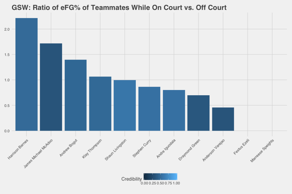
Interestingly, the results don’t look too great for some of the stars on the Warriors. The best values come from either players who didn’t get much playing time (McAdoo and Bogut) and Harrison B arnes, who lives in the shadows of Curry, Thompson, and Green. The results for McAdoo and Bogut could simply be chance error due to the small sample size (credibility isn’t very good for any of the GSW players due to their skewed rotation) or the fact that they were probably playing during times when Cleveland also had their reserves in the game. The results for Barnes are more interesting, though. As a starter, he probably played the majority of his time with other starters. Yet his ratio is much better than the rest of the starters. That could be worth investigating.
For now, though, I’ll wrap up this little analysis. I think there’s a sufficient level of granularity in this data to allow me to waste hours and hours nerding out, so I’ll be purchasing the BigDataBall subscription for the upcoming season and the data for historical seasons. I’ll be blogging more about random play-by-play analyses over the course of the season, so stay tuned!
